Algorithm at a glance!

Algorithms are at the heart of computer science and play a crucial role in solving problems across various domains. An algorithm can be defined as a well-defined sequence of steps or instructions designed to perform a specific task or solve a particular problem. Algorithms are the driving force behind computer programs, enabling them to process data and perform computations efficiently.

Algorithms have several key characteristics that distinguish them from random sets of instructions. They must be well-defined, meaning that each step in the algorithm should be clear and unambiguous. Algorithms also require input, which is the data or information provided to the algorithm, and produce output, which is the solution or result obtained after executing the algorithm's steps. Additionally, algorithms must be finite, meaning they should terminate after a finite number of steps, and effective, meaning that each step should be executable and lead towards the desired solution.

Algorithmic thinking is a fundamental problem-solving skill that involves breaking down complex problems into smaller, manageable steps and devising a logical sequence of instructions to solve them. This thought process is essential in programming and computing but also has applications in various other fields, such as mathematics, biology, and finance.

When designing algorithms, it is crucial to consider their correctness and efficiency. Correctness refers to the ability of an algorithm to produce the desired output for any valid input, while efficiency measures how well an algorithm utilises computational resources, such as time and memory. Algorithm analysis techniques, like time and space complexity analysis, help evaluate the performance of algorithms and make informed decisions about their suitability for specific problems.

There are numerous types of algorithms, each designed to solve a particular class of problems. Some common examples include searching algorithms (linear search, binary search), sorting algorithms (bubble sort, merge sort, quicksort), graph algorithms (shortest path algorithms, minimum spanning tree algorithms), and algorithmic paradigms like divide and conquer, greedy algorithms, and dynamic programming.

Algorithms have numerous applications across various disciplines, including computer science (data structures, databases, computer networks, artificial intelligence), mathematics (numerical analysis, cryptography), biology (genomic sequence analysis, protein structure prediction), finance (portfolio optimisation, risk analysis), and logistics (routing and scheduling problems).

The study of algorithms not only equips students with problem-solving skills but also fosters computational thinking, a way of approaching problems that involves breaking them down into smaller parts, identifying patterns, and developing step-by-step solutions that can be executed by a computer or human. This mind-set is valuable not only in computer science but also in other fields where complex problem-solving is required.

Algorithms are the backbone of computing and problem-solving, providing a systematic approach to tackling complex challenges. Understanding algorithms, their design principles, and their analysis is crucial for both computer science and non-computer science students, as it equips them with valuable problem-solving skills and a computational thinking mind-set applicable across various domains.

Algorithm Analysis and Complexity

Analysing the efficiency of algorithms is a critical aspect of algorithm design and implementation. As the size of input data or the problem instances grow, the performance of an algorithm can vary significantly. Algorithm analysis provides a systematic way to evaluate the efficiency of algorithms and helps in making informed decisions about their suitability for specific problems.

One of the fundamental concepts in algorithm analysis is time complexity, which measures the amount of time an algorithm takes to execute as a function of the input size. Time complexity is typically expressed using Big O notation, which provides an upper bound on the growth rate of the algorithm's running time. For example, an algorithm with a time complexity of O(n) will have a running time that grows linearly with the input size, while an algorithm with a time complexity of O(n^2) will have a running time that grows quadratically.

Space complexity is another important aspect of algorithm analysis, which measures the amount of memory or storage space an algorithm requires as a function of the input size. Like time complexity, space complexity is also expressed using Big O notation. An algorithm with a space complexity of O(1) uses a constant amount of memory, regardless of the input size, while an algorithm with a space complexity of O(n) requires memory that grows linearly with the input size.

Understanding the time and space complexities of algorithms is crucial for several reasons:

1. Performance Evaluation: By analysing the time and space complexities, you can predict how an algorithm will perform for different input sizes and make informed decisions about which algorithm to use for a particular problem.

2. Scalability Assessment: Some algorithms may perform well for small input sizes but become inefficient or impractical for larger inputs. Complexity analysis helps identify such scalability issues and guides the selection of appropriate algorithms for different problem scales.

3. Resource Optimisation: In resource-constrained environments, such as embedded systems or mobile devices, understanding the space complexity of an algorithm is essential to ensure efficient memory usage.

4. Comparative Analysis: Complexity analysis provides a common ground for comparing the efficiency of different algorithms designed to solve the same problem. This information can guide the selection of the most appropriate algorithm for a given scenario.

It's important to note that algorithm analysis provides an asymptotic analysis, which means it focuses on the behaviour of the algorithm as the input size grows towards infinity. While actual running times may vary depending on factors like hardware, programming language, and implementation details, asymptotic analysis provides a reliable way to compare the theoretical efficiency of algorithms.

In addition to time and space complexity, algorithm analysis may also consider other factors, such as the best-case, average-case, and worst-case scenarios, as well as the trade-offs between time and space complexities. Understanding these concepts is essential for designing efficient algorithms and making informed decisions about their implementation and usage in various applications.

Data Structures and Abstract Data Types

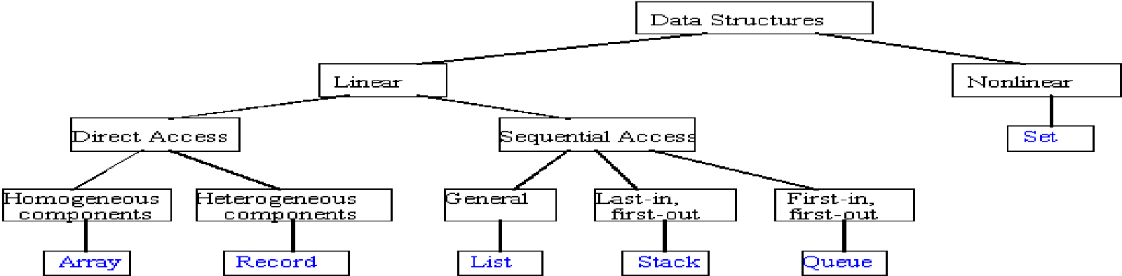
Data structures are fundamental building blocks in computer science and algorithm design. They are ways of organising and storing data in a computer's memory so that it can be efficiently accessed and manipulated by algorithms. The choice of data structure used in an algorithm can significantly impact its performance, memory usage, and overall efficiency.

Abstract Data Types (ADTs) are conceptual models or blueprints for data structures. They define the behaviour and operations that a data structure should support without specifying the implementation details. ADTs provide a way to encapsulate the internal representation of data and expose only the necessary operations to the user, promoting code modularity and reusability.

Some common examples of data structures and their corresponding ADTs include:

1. Arrays and Lists: Arrays and lists are linear data structures that store a collection of elements in a sequential manner. The ADT for arrays and lists typically defines operations such as accessing elements by index, inserting new elements, removing elements, and searching for elements.

2. Stacks and Queues: Stacks and Queues are linear data structures that follow specific rules for inserting and removing elements. The stack ADT defines operations like push (inserting an element at the top), pop (removing the top element), and peek (accessing the top element without removal). The queue ADT defines operations like enqueue (inserting an element at the rear), dequeue (removing the element from the front), and front (accessing the front element without removal).

3. Trees: Trees are hierarchical data structures where elements are organized in a parent-child relationship. The tree ADT defines operations like inserting nodes, deleting nodes, searching for nodes, and traversing the tree in different orders (e.g., pre-order, in-order, post-order).

4. Graphs: Graphs are non-linear data structures that consist of nodes (vertices) connected by edges. The graph ADT defines operations like adding vertices, adding edges, removing vertices, removing edges, and traversing the graph using algorithms like breadth-first search (BFS) or depth-first search (DFS).

5. Hash Tables: Hash tables are data structures that store key-value pairs and provide efficient lookup, insertion, and deletion operations. The hash table ADT defines operations like insert (adding a key-value pair), delete (removing a key-value pair), and search (finding the value associated with a given key).

The choice of data structure depends on the specific requirements of the problem at hand, such as the need for random access, insertion/deletion efficiency, or efficient search operations. ADTs provide a standardised interface for working with data structures, allowing programmers to focus on the logical operations without worrying about the underlying implementation details.

Understanding data structures and ADTs is crucial for designing efficient algorithms and writing optimised code. By selecting the appropriate data structure for a given problem, algorithms can achieve better performance, memory utilisation, and overall efficiency, making them more scalable and capable of handling larger problem instances.

Searching Algorithms

Searching is a fundamental operation in computer science and programming, which involves finding the location or existence of a particular element within a data structure or a collection of data. Searching algorithms are designed to efficiently locate the desired element or determine its absence from the given data set. These algorithms play a crucial role in various applications, such as databases, information retrieval systems, and data processing tasks.

Some of the most common searching algorithms include:

1. Linear Search: Linear search is a simple algorithm that sequentially checks each element in the data structure until the desired element is found or the entire data structure is traversed. It has a time complexity of O(n) in the worst case, where n is the size of the data structure. Linear search is efficient for small data sets or unsorted collections but becomes inefficient for large data sets.

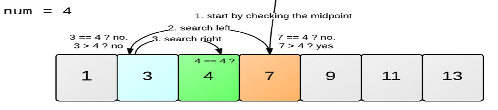
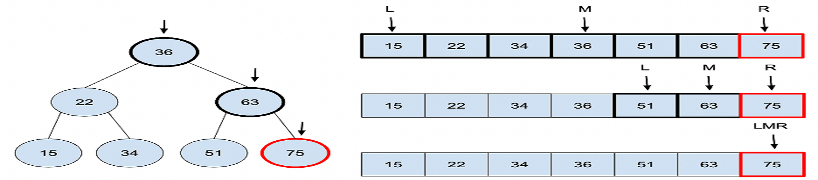
2. Binary Search: Binary search is an efficient algorithm for finding an element in a sorted array or list. It works by repeatedly dividing the search interval in half until the desired element is found or it is determined that the element is not present. Binary search has a time complexity of O(log n) in the average and best cases, making it highly efficient for large sorted data sets.

3. Depth-First Search (DFS): Depth-First Search is an algorithm used for traversing or searching tree or graph data structures. It explores as far as possible along each branch before backtracking and exploring the next branch. DFS can be implemented using recursion or an explicit stack. Its time complexity depends on the structure of the tree or graph being searched.

4. Breadth-First Search (BFS): Breadth-First Search is another algorithm used for traversing or searching tree or graph data structures. Unlike DFS, it explores all the nodes at the current depth level before moving on to the next depth level. BFS can be implemented using a queue data structure. Its time complexity also depends on the structure of the tree or graph being searched.

5. Hash-based Search: Hash-based search is a technique used for searching elements in a hash table or dictionary data structure. It involves computing a hash value (a fixed-size integer) from the key and using that hash value to index into a bucket or slot in the hash table. Hash-based search has an average-case time complexity of O(1), making it extremely efficient for lookup operations.

The choice of a searching algorithm depends on several factors, including the size of the data set, whether the data is sorted or unsorted, the data structure being used, and the specific requirements of the application. For example, if the data set is small and unsorted, linear search may be the simplest choice. If the data set is large and sorted, binary search is often the most efficient option. For searching in tree or graph data structures, algorithms like DFS and BFS are commonly used.

Searching algorithms are not only important in their own right but also serve as building blocks for more complex algorithms and data processing tasks. Understanding the strengths and limitations of different searching algorithms is crucial for designing efficient solutions to various computational problems.

Greedy Algorithms

Greedy algorithms are a class of algorithms that follow the problem-solving heuristic of making the locally optimal choice at each stage with the hope of finding a global optimum. In other words, a greedy algorithm makes the best choice at the current step based on the available information, without considering the consequences of that choice on future steps.

The greedy approach is based on the principle of making choices that seem best at the moment and hoping that these choices will lead to the overall optimal solution. This approach is particularly useful when the problem can be broken down into smaller subproblems, and the optimal solution to the overall problem can be constructed from the optimal solutions to the subproblems.

Some key characteristics of greedy algorithms include:

1. Greedy Choice Property: At each step, the algorithm makes a greedy choice that appears to be the best at that moment, without considering the impact on future steps.

2. Optimal Substructure: The problem exhibits optimal substructure, meaning that the optimal solution can be constructed from optimal solutions to its subproblems.

3. Greedy algorithms are typically faster and more efficient than many other algorithms, as they don't require exploring all possible solutions.

Examples of greedy algorithms include:

1. Kruskal's Algorithm: Used to find the minimum spanning tree of a weighted undirected graph. It greedily selects the edges with the lowest weights until it forms a minimum spanning tree.
2. Prim's Algorithm: Another algorithm for finding the minimum spanning tree of a weighted undirected graph. It starts with an arbitrary vertex and greedily adds the next closest vertex to the growing tree.
3. Huffman Coding: A greedy algorithm used for data compression. It constructs an optimal prefix code tree by iteratively merging the two smallest-frequency nodes.
4. Job Scheduling: Greedy algorithms can be used to schedule jobs or tasks based on priorities or deadlines, where the algorithm greedily selects the job or task with the highest priority or earliest deadline.
5. Dijkstra's Algorithm: While not a purely greedy algorithm, Dijkstra's algorithm for finding the shortest path in a weighted graph uses a greedy approach by selecting the vertex with the minimum distance from the source at each iteration.

Greedy algorithms are not always guaranteed to produce the optimal solution, as their greedy choices may lead to a suboptimal solution in some cases. However, for many problems where the greedy approach works, these algorithms can provide efficient and practical solutions.

It's important to note that the correctness and optimality of a greedy algorithm depend on the problem satisfying certain properties, such as the greedy choice property and optimal substructure. Before applying a greedy approach, it is crucial to analyse the problem thoroughly and ensure that the greedy strategy will lead to the desired optimal solution.

Divide and Conquer Algorithms

The divide and conquer algorithm design paradigm is a powerful problem-solving technique that involves breaking down a complex problem into smaller sub-problems, solving each sub-problem independently, and then combining the solutions to the sub-problems to obtain the final solution to the original problem.

The divide and conquer approach typically follows these three steps:

1. Divide: In this step, the original problem is divided into smaller sub-problems that are similar in nature but smaller in size.
2. Conquer: Each sub-problem is solved recursively, often using the same divide and conquer approach. If the sub-problems are small enough, they can be solved directly using a base case solution.
3. Combine: The solutions to the sub-problems are combined to form the final solution to the original problem.

The key advantages of the divide and conquer approach include:

1. Efficiency: Many divide and conquer algorithms have a time complexity of O(n log n), which is more efficient than the brute force approach of O(n^2) or higher for many problems.
2. Parallelisation: Since the sub-problems are independent, they can be solved in parallel, leading to faster execution times on parallel processing systems.
3. Memory usage: Recursive solutions in divide and conquer algorithms often have better space complexity compared to iterative solutions, as they don't require additional data structures for storing intermediate results.

Some classic examples of divide and conquer algorithms include:

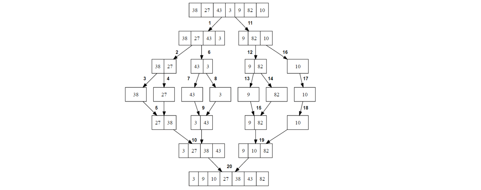
1. Merge Sort: An efficient sorting algorithm that divides the input array into two halves, recursively sorts them, and then merges the sorted halves to produce the final sorted array.
2. Quicksort: Another efficient sorting algorithm that partitions the input array around a pivot element, recursively sorts the two partitions, and then combines them.
3. Strassen's Algorithm: An algorithm for matrix multiplication that recursively breaks down the matrix multiplication into smaller sub-problems, solves them, and combines the results.
4. Closest Pair of Points: An algorithm that finds the closest pair of points in a set of points by dividing the set into two halves, solving the sub-problems recursively, and then combining the solutions.
5. Integer Multiplication: Algorithms like Karatsuba's algorithm use the divide and conquer approach to multiply large integers more efficiently than the traditional long multiplication method.

The divide and conquer paradigm can be applied to a wide range of problems, including sorting, searching, numerical computation, and optimization problems. However, not all problems are suitable for this approach, as they may not exhibit the necessary properties, such as the ability to divide the problem into smaller sub-problems or the existence of a base case.

When designing divide and conquer algorithms, it is crucial to analyse the time and space complexity carefully, as the overhead of dividing and combining the sub-problems can sometimes outweigh the benefits of the recursive approach.

Overall, the divide and conquer algorithm design paradigm is a powerful and versatile technique that has contributed to the development of many efficient algorithms in computer science and other fields.

Dynamic Programming

Dynamic Programming (DP) is a powerful algorithmic technique used to solve a complex problem by breaking it down into simpler sub-problems and efficiently solving each sub-problem only once. It is based on the principle of storing the solutions to sub-problems and reusing them whenever needed, instead of recomputing them multiple times.

The key idea behind dynamic programming is to avoid redundant calculations by **memoising (storing) the results of sub-problems and using them to solve larger problems. This approach is particularly useful when the same sub-problems are encountered multiple times in the overall problem-solving process.

Dynamic programming typically follows these steps:

1. Identify the sub-problems: Break down the original problem into smaller sub-problems that can be solved independently.
2. Define the base cases: Specify the base cases or the simplest instances of the problem that can be solved directly.
3. Write a recurrence relation: Express the solution to the original problem in terms of the solutions to its sub-problems using a recurrence relation.
4. Memoise or tabulate the sub-problem solutions: Store the solutions to sub-problems in a data structure (e.g., an array or a dictionary) to avoid redundant calculations.
5. Solve the original problem by combining the sub-problem solutions using the recurrence relation.

Dynamic programming can be implemented using two main techniques: top-down (memoisation) or bottom-up (tabulation). In the top-down approach, the problem is solved recursively, and the results of sub-problems are stored in a memoisation table to avoid redundant calculations. In the bottom-up approach, a tabulation table is filled in a specific order, starting with the base cases and building up the solutions to larger sub-problems.

**In computing, memoization or memoisation is an optimisation technique used primarily to speed up computer programs by storing the results of expensive function calls to pure functions and returning the cached result when the same inputs occur again. [Wikipedia]

Some classic examples of problems that can be solved using dynamic programming include:

1. Fibonacci Series: Computing the nth Fibonacci number efficiently.
2. Knapsack Problem: Determining the maximum value that can be obtained by filling a knapsack with a given weight capacity and a set of items with weights and values.
3. Longest Common Subsequence (LCS): Finding the longest common subsequence between two strings.
4. Matrix Chain Multiplication: Finding the optimal way to multiply a sequence of matrices to minimize the number of operations.
5. Shortest Path Problems: Finding the shortest path between two nodes in a weighted graph using algorithms like the Bellman-Ford algorithm.

Dynamic programming is widely used in various domains, including computer science, operations research, economics, and bioinformatics, due to its ability to solve complex optimisation problems efficiently.

It is important to note that not all problems can be solved using dynamic programming. For a problem to be suitable for dynamic programming, it must exhibit two key properties: optimal substructure and overlapping sub-problems. Optimal substructure means that the optimal solution to the problem can be constructed from the optimal solutions to its sub-problems. Overlapping sub-problems means that the same sub-problems are encountered multiple times during the problem-solving process.

While dynamic programming can provide efficient solutions to many problems, it often comes at the cost of increased memory usage due to the need to store the solutions to sub-problems. Therefore, a careful analysis of time and space complexities is essential when designing dynamic programming algorithms.

Graph Algorithms

Graphs are a fundamental data structure in computer science that represent relationships between objects or entities. They consist of nodes (vertices) and edges that connect these nodes. Graph algorithms are a set of techniques and procedures designed to solve problems related to graphs, such as finding paths, traversing nodes, or identifying specific properties or patterns within the graph structure.

Some of the most important graph algorithms include:

1. Graph Traversal Algorithms:

a. Depth-First Search (DFS): This algorithm explores as far as possible along each branch before backtracking and exploring the next branch. It can be used to detect cycles, find connected components, and solve problems like topological sorting and maze traversal.

b. Breadth-First Search (BFS): This algorithm explores all the neighbouring nodes at the current depth level before moving on to the next depth level. It is commonly used for finding the shortest path between two nodes in an unweighted graph and for solving problems like the minimum spanning tree and connected components.

2. Shortest Path Algorithms:

a. Dijkstra's Algorithm: This algorithm finds the shortest path between a source node and all other nodes in a weighted graph with non-negative edge weights. It is widely used in routing algorithms, network optimisation, and path planning problems.

b. Bellman-Ford Algorithm: This algorithm can handle negative edge weights and can detect negative cycles in a weighted graph. It is useful in scenarios where edge weights can be negative, such as in network routing with link costs.

c. Floyd-Warshall Algorithm: This algorithm finds the shortest paths between all pairs of nodes in a weighted graph. It is particularly useful when multiple source-destination pairs need to be considered, such as in routing and network analysis.

3. Minimum Spanning Tree Algorithms:

a. Kruskal's Algorithm: This algorithm finds the minimum spanning tree (MST) of a weighted, undirected graph. It builds the MST by greedily selecting the edges with the lowest weights, avoiding cycles.

b. Prim's Algorithm: This algorithm also finds the MST of a weighted, undirected graph. It starts with an arbitrary node and greedily adds the next closest node to the growing tree.

4. Topological Sorting:

a. Used to find a linear ordering of nodes in a directed acyclic graph (DAG), such that for every directed edge from node A to node B, node A appears before node B in the ordering. This algorithm is useful in scheduling tasks with dependencies or resolving circular dependencies in software systems.

5. Network Flow Algorithms:

a. Ford-Fulkerson Algorithm: This algorithm is used to find the maximum flow in a flow network, which can represent various real-world scenarios like traffic flow, communication networks, and supply chain optimisation.

b. Edmonds-Karp Algorithm: An implementation of the Ford-Fulkerson algorithm that uses breadth-first search to find the augmenting paths, making it more efficient for certain types of networks.

Graph algorithms have numerous applications in various fields, including computer networks (routing and traffic flow), social networks (analysing relationships and recommender systems), bioinformatics (analysing protein interactions and gene sequences), transportation and logistics (route planning and optimization), and many more.

The choice of a specific graph algorithm depends on the problem at hand, the properties of the graph (e.g., directed or undirected, weighted or unweighted), and the desired output or optimisation criteria. Many graph algorithms have variations and optimisations to improve their performance or handle specific problem constraints.

Understanding graph algorithms is crucial for solving complex problems involving relationships, networks, and interconnected systems. They provide powerful tools for analysing, optimising, and understanding the intricate structures and patterns present in many real-world scenarios.

Advanced Algorithms and Techniques

While the basic algorithms and techniques covered earlier form the foundation of algorithm design, there are several advanced algorithms and techniques that address more complex problems or provide specialised solutions. These advanced techniques often involve sophisticated mathematical concepts, theoretical frameworks, or specialised problem-solving approaches. Some of these advanced algorithms and techniques include:

1. Randomised Algorithms: Randomised algorithms incorporate randomness into their logic and decision-making process. They make random choices at certain points during execution, allowing them to explore different solution paths and potentially improve their efficiency or accuracy. Examples include randomised quicksort, randomised primality testing, and randomised min-cut algorithms.
2. Parallel and Distributed Algorithms: With the advent of multi-core processors and distributed computing systems, algorithms designed to leverage parallel and distributed processing have become increasingly important. These algorithms divide the computational workload among multiple processors or machines, aiming to solve problems more efficiently or tackle larger problem instances. Examples include parallel sorting algorithms, parallel graph algorithms, and distributed database query processing algorithms.
3. Approximation Algorithms: For certain computationally hard problems, finding an exact optimal solution may be infeasible or impractical within reasonable time and resource constraints. Approximation algorithms trade off the precision of the solution for improved efficiency, providing a near-optimal solution that is within a provable bound of the optimal solution. Examples include approximation algorithms for the traveling salesman problem, bin packing, and vertex cover problems.
4. Geometric Algorithms: Geometric algorithms deal with problems involving geometric objects, such as points, lines, polygons, and polyhedra. These algorithms are used in areas like computer graphics, computer-aided design (CAD), robotics, and geographic information systems (GIS). Examples include convex hull algorithms, line segment intersection algorithms, and point location algorithms.
5. String Matching and Computational Biology Algorithms: These algorithms focus on processing and analysing string data, with applications in areas like text processing, data compression, and computational biology. Examples include string matching algorithms (e.g., Knuth-Morris-Pratt, Boyer-Moore), sequence alignment algorithms (e.g., Needleman-Wunsch, Smith-Waterman), and genome assembly algorithms.
6. Cryptographic Algorithms: Cryptographic algorithms are used for secure communication, data encryption, and digital signatures. They rely on advanced mathematical concepts like number theory, finite fields, and combinatorics. Examples include public-key cryptography algorithms (e.g., RSA, Diffie-Hellman), symmetric-key cryptography algorithms (e.g., AES, DES), and hash functions (e.g., SHA-256, MD5).
7. Quantum Algorithms: With the emergence of quantum computing, researchers have developed quantum algorithms that leverage the principles of quantum mechanics to solve certain problems more efficiently than classical algorithms. Examples include Shor's algorithm for integer factorization, Grover's algorithm for unstructured search, and quantum simulation algorithms.

These advanced algorithms and techniques are often studied and applied in research areas such as theoretical computer science, cryptography, computational biology, and quantum computing. They may involve complex mathematical concepts, probabilistic models, or specialised problem-solving approaches tailored to specific domains or problem classes.

While some of these advanced techniques may not be immediately applicable in all contexts, understanding their underlying principles and potential applications can provide valuable insights and inspire novel approaches to solving complex problems across various fields.

Algorithm Design Techniques

Algorithm design is a fundamental aspect of computer science and problem-solving. It involves developing step-by-step procedures or strategies to solve computational problems efficiently and accurately. Over the years, various algorithm design techniques have been developed to tackle different types of problems and optimise specific aspects of algorithms, such as time complexity, space complexity, or problem-specific constraints. Here are some of the most common algorithm design techniques:

1. Brute Force: The brute force technique involves enumerating all possible solutions to a problem and checking each one to find the optimal solution. While simple to implement, brute force algorithms can be inefficient for large problem instances due to their high time and space complexity. However, they can be useful in certain scenarios, such as solving small instances or serving as a baseline for evaluating more sophisticated algorithms.
2. Greedy Approach: Greedy algorithms follow the principle of making the locally optimal choice at each stage, with the hope of finding the global optimum. These algorithms make the best choice at the current step based on the available information, without considering the consequences of that choice on future steps. Greedy algorithms are often efficient and can provide optimal solutions for problems exhibiting the greedy choice property and optimal substructure.
3. Divide and Conquer: The divide and conquer technique involves breaking down a complex problem into smaller sub-problems of the same type, solving each sub-problem independently, and then combining the solutions to the sub-problems to obtain the final solution. This approach is particularly useful for problems that exhibit optimal substructure and can be solved recursively. Many efficient algorithms, such as merge sort and Strassen's algorithm, are based on the divide and conquer technique.
4. Dynamic Programming: Dynamic programming is a technique that solves complex problems by breaking them down into simpler sub-problems, solving each sub-problem once, and storing the solutions for reuse. It is based on the principle of avoiding redundant calculations by memoising or tabulating the solutions to sub-problems. Dynamic programming is applicable to problems exhibiting optimal substructure and overlapping sub-problems, such as the knapsack problem, longest common subsequence, and shortest path problems.
5. Backtracking: Backtracking is a general algorithmic technique that considers searching every possible combination in order to solve a computational problem. It incrementally builds candidates to the solutions and abandons a candidate ("backtracking") as soon as it determines that the candidate cannot possibly be completed to a valid solution. Backtracking is used in problems involving constraint satisfaction, such as N-queens, Sudoku solvers, and graph colouring.
6. Branch and Bound: Branch and bound is an optimisation technique used to solve computationally difficult problems, such as integer programming and combinatorial optimisation problems. It involves systematically enumerating candidate solutions by means of a state space tree and using upper and lower bounds to prune away branches that cannot possibly contain the optimal solution.
7. Randomised Algorithms: Randomised algorithms incorporate randomness into their logic and decision-making process. They make random choices at certain points during execution, allowing them to explore different solution paths and potentially improve their efficiency or accuracy. Randomised algorithms are used in areas such as primality testing, hashing, and randomized optimization.

These algorithm design techniques are not mutually exclusive, and often a combination of techniques may be employed to design efficient and effective algorithms for specific problems. The choice of technique depends on the nature of the problem, the desired time and space complexity, and any additional constraints or requirements.

Familiarity with these algorithm design techniques is essential for computer science students and professionals, as it equips them with a diverse set of problem-solving strategies and enables them to design efficient and optimized algorithms for a wide range of computational problems.

Practical Applications and Case Studies

Algorithms are not just theoretical constructs; they have numerous practical applications in various domains of our daily lives. Understanding how algorithms are applied in real-world scenarios can help both computer science and non-computer science students appreciate their significance and impact. Here are some practical applications and case studies of algorithms:

1. Web Search Engines: Search engines like Google, Bing, and DuckDuckGo rely heavily on algorithms to crawl, index, and rank web pages. Algorithms like PageRank (used by Google) and web crawling algorithms play a crucial role in determining the relevance and ordering of search results.
2. Routing and Navigation: Algorithms like Dijkstra's algorithm and the A* search algorithm are used in routing and navigation applications, such as Google Maps and GPS systems, to find the shortest or most efficient routes between locations, taking into account factors like traffic conditions and road networks.
3. Recommendation Systems: Online platforms like Netflix, Amazon, and Spotify use collaborative filtering algorithms and other recommendation algorithms to suggest movies, products, or music based on user preferences, ratings, and browsing histories.
4. Compression Algorithms: Data compression algorithms like Huffman coding and arithmetic coding are used in various applications, including image and video compression (e.g., JPEG and MPEG), file compression (e.g., ZIP and RAR), and data transmission, to reduce the size of data and improve efficiency.
5. Cryptography: Algorithms like RSA, AES, and SHA are at the heart of modern cryptography, ensuring secure communication and data protection in applications like online banking, e-commerce, and secure messaging.
6. Machine Learning and Artificial Intelligence: Many algorithms are used in machine learning and artificial intelligence, such as decision tree algorithms, support vector machines, and neural network algorithms. These algorithms are used in various applications, including image recognition, natural language processing, and predictive modelling.
7. Computational Biology: Algorithms like sequence alignment algorithms (e.g., Needleman-Wunsch, Smith-Waterman) and genome assembly algorithms play a crucial role in bioinformatics and computational biology, helping researchers analyse and understand genetic data, protein structures, and biological processes.
8. Scheduling and Optimisation: Algorithms like the Hungarian algorithm, the simplex algorithm, and various scheduling algorithms are used in operations research and logistics to optimise resource allocation, scheduling, and routing problems in industries like manufacturing, transportation, and supply chain management.
9. Computer Graphics and Gaming: Algorithms like rendering algorithms, collision detection algorithms, and pathfinding algorithms (e.g., A* search) are essential components of computer graphics and gaming applications, enabling realistic rendering, smooth character movement, and efficient level design.
10. Financial and Business Applications: Algorithms like the Markowitz portfolio optimization algorithm, option pricing models (e.g., Black-Scholes model), and various data mining algorithms are used in finance and business for tasks such as portfolio management, risk analysis, and market trend prediction.

These are just a few examples of the numerous practical applications of algorithms across various domains. As technology continues to evolve, the role of algorithms in solving real-world problems and driving innovation will only become more significant. By studying algorithms and their practical applications, students can develop a deeper understanding of their impact and potential contributions to society.